


This version (01 Nov 2021 18:28) was approved by Mark Thoren.The Previously approved version (01 Nov 2021 18:16) is available.
Table of Contents
Activity: Transmission Lines and Standing Waves
Objective:
The objective of this exercise is to develop a basic understanding of the operation of an electrical transmission line and to explore the effects of “standing waves” in such a line. Transmission lines can be a daunting subject when they are first encountered. But this exercise will draw some analogies to acoustic transmission lines, examples of which are wind instruments (trombone, pipe organ, jug band jug), and even an echo along a hallway with a wall at one end. If you clap in a hallway, you may hear an echo of your own clap a perceptible time later. What if you walk closer to the closed end so that the echo is sooner and sooner after the incident clap? What do you think would happen if the reflected wave encountered the forward wave before it had ended? You would end up with a “standing wave”. It is possible to set up such an experiment in a controlled and extreme way, with a 100-watt “clap” directed down a 2m long, 10cm diameter “hallway”, as shown in this video:
Electrical transmission lines, especially short ones, require high-speed (and expensive) test equipment to characterize. Fortunately, LTspice can simulate arbitrarily long transmission lines with time delays of milliseconds and longer, with corresponding resonant frequencies in the audio range. This exercise will start with LTspice simulations, then conclude with several acoustical experiments and their simulated electrical equivalents.
Background
Transmission Lines – General Information
A transmission line is defined as a system of conductors (wires, waveguides, coaxial cables), suitable for conducting electric power signals between two or more terminals. [McGraw-Hill Dictionary of Scientific and Technical Terms].
To send an electrical signal to a distant load, two wires are required. (The wires need not be symmetrical - in fact one wire can be the Earth itself.) Since two conductors are, by definition, a capacitor, this implies that each section of a transmission line has some capacitance. On the other hand, as an inductor is defined essentially as a loop of wire, each section of the line also has an inductance. In reality, each “section” of the line can be thoght of as an infinitesimally small unit capacitance and inductance. A “lumped” model of a transmission line can also be constructed with discrete inductors and capacitors as shown in Figure 1. (Naturally, the model is more accurate when a large number of smaller capacitors and inductors are used - at the expense of complexity and size.) Suppose a constant DC voltage is suddenly applied to one end of the transmission line. The capacitance and inductance prevent the signal from travelling down the line instantaneously.

Figure 1. Lumped Element equivalent of a transmission line
Voltage applied between two conductors creates an electric field between them. Equation 1 implies that the current drawn from the voltage source would be proportional to the voltage’s rate of change over time. In consonance with said equation, an instant rise in applied voltage, results in an infinite charging current. Nonetheless, the current drawn will not be infinite because of the series impedance, due to line inductance. Each wire from our pair develops a magnetic field as it carries charging current for the capacitance between the wires, dropping voltage according to equation 2. This voltage drop limits the voltage rate of change across the distributed capacitance, preventing the current from ever reaching an infinite magnitude. Thus, the wires are no longer simple conductors - they are themselves a circuit component called a transmission line, with their own characteristics. When voltage is suddenly applied, both a current wave and a voltage wave propagate along the line’s length at a significant fraction of the speed of light.
Equation 1:
Where:
i is the instantaneous current through the capacitor;
C is the capacitance in Farads;
is the instantaneous rate of voltage change, volts per second.
Equation 2:
Where:
v is the instantaneous voltage across the inductor;
L is the inductance in Henrys;
is the instantaneous rate of current change, amps per second.
The physical construction of a transmission line varies widely depending on the application. There are several different types of electrical transmission lines such as coaxial line (figure 2), two-wire line (figure 3), parallel-plate line, strip line, microstrip line, coplanar waveguide.
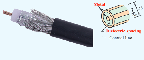
Figure 2. Coaxial line

Figure 3. Two-wire line
A common example of a 2-wire transmission line is unshielded twisted pair (UTP) ethernet cable everyone is familiar with. If the twisted pair is surrounded by a solid dielectric (or “shield”), the line becomes a shielded pair transmission line (STP). Both cables are shown in figure 4. When using UTP transmission lines, several parameters need to be considered: attenuation (amount of loss in signal’s strength as it travels down a wire), crosstalk (unwanted coupling caused by overlapping electric and magnetic fields), near-end crosstalk (measure of level of signal coupling within a cable). A visual representation of the latter is depicted in figure 5. There are a couple of advantages to using the shielded pair cable, such as:
- Conductors are contained within in a copper braid shield, which isolates from external noise and prevents radiating and interfering with other systems.
- Near-end crosstalk between pairs in a multi-pair cable is reduced.

Figure 4: UTP and STP cables

Figure 5: Near-end crosstalk
Characteristic Impedance
Characteristic/ natural impedance refers to the equivalent resistance of a transmission line if it were infinitely long, owing to distributed capacitance and inductance, as the voltage and current waves travel along its length at a propagation velocity equal to some large fraction of the speed of light (3.0*10^8 m/s) Suppose the spacing between the two conductors is expanded. Under this condition, the distributed capacitance will decrease, while the distributed inductance will increase, as there is less cancelation between two opposing magnetic fields. Naturally, by bringing the capacitor plates (the two conductors) closer together, the antagonistic effect is obtained: increased parallel capacitance and decreased series inductance. Hence, one can note that the characteristic impedance of a transmission line increases as there is greater space between conductors. To calculate the natural impedance of a given transmission line, with known parameters, the following formula shown in equation 3 is to be used. This shows that characteristic impedance is purely a function of the capacitance and inductance distributed along the lines length and it would exist even if the dielectric were perfect (infinite parallel resistance) and the wires superconducting (zero series resistance).
Equation 3:
where characteristic impedance of line;
L – inductance per unit length of line;
C – capacitance per unit length of line.
In an actual transmission line, the inductance and capacitance, and therefore the characteristic impedance, are functions of the geometry. The characteristic impedance of a parallel pair transmission line is shown in Equation 4, and the characteristic impedance of a coaxial transmission line is shown in Equation 5.
Equation 4:
Where:
k is the relative permittivity of the dielectric (unity for air)
d is the center-to-center distance between conductors in mm
r is the radius of the conductors in mm
Equation 5:
Where:
k is the relative permittivity of the dielectric (unity for air)
d1 is the inside diameter of the outer conductor in mm
d2 is the outside diameter of the inner conductor in mm
Incident and Reflected Waves
A signal which travels from the source-end of the transmission line to the load-end, is called an incident wave, while a wave which propagates in the opposite direction is defined as a reflected wave. Leaving the end of a transmission line open-circuited (unconnected), results in a “pile-up” of electric charge carriers at the line’s end, as the incident current wave propagating along the line cannot flow where there is no continuing path. When this electric charge carriers propagates back as a reflected wave, current at the source ceases, and the line becomes a simple open circuit. A similar event occurs when the line’s end is short-circuited: the voltage wave front is reflected to the source, as it reaches the end of the line, since voltage cannot exist between two electrically common points. As the reflected wave arrives at the source-end, the source views the entire transmission line as a short-circuit. Reflections may also appear when connecting two transmission lines, whose characteristic impedance differ. When dealing with signal transmission, it is important to state that the ideal situation would be for the entirety of the original signal’s energy to travel from source to load, and then be completely absorbed or dissipated by the load, with the maximum power transfer. It is then obvious that both loss along the line and reflected waves are undesirable.
Reflections may be avoided, if the load’s impedance matches the characteristic impedance of the transmission line, making the line seem infinitely long, as far as the source is concerned. This is due to a resistor’s ability to continuously dissipate energy, just as an infinitely long transmission line would eternally absorb energy. Should the source’s impedance be exactly equal to the line’s, a reflected wave, which reaches the source, would be dissipated entirely. However, if these two quantities do not match, the wave is partially re-reflected to the load end of the line, as another incident wave.

Figure 6. Free end (left) and fixed end (right) reflection of incident wave
Wavelength and Transmission Line Length
The wavelength of a signal is defined as the distance between successive crests (or troughgs) of a wave. Equation 6 shows the relationship between wavelength, frequency, and velocity.
Equation 6:
Where:
v is the velocity of propagation
f is the signal frequency
λ is the wavelength
Whether a conductor can be considered a transmission line or not depends on the frequency content of the signal and the propagation speed along the conductor. One generally accepted rule of thumb is that if a transmission line is more than about 1/10 of a wavelength, then propagation effects should be considered. Cat-6 Ethernet cable has a typical velocity factor of about 0.65, or 1.95e8 meters per second. A 2m cable thus represents 1 wavelength at 97.5MHz. This is qualitatively a “high” frequency - it's well above audio, and in the middle of the FM broadcast band. But remember the rule of thumb - at 97MHz the 2m cable is definitely a transmission line. But transmission line effects - reflections and standing waves that can potentially corrupt communications - will begin to take effect around 9.7MHz!
9.7MHz may still sound “fast”, but consider a common situation where one microcontroller (such as an Arduino or Raspberry Pi) is communicating with another. 2 meters is “not too far” away, so perhaps the 2m Ethernet cable would work for typical UART Baud rates - 9600 Baud, 115200 Baud, or even a bit faster.
But other “medium speed” protocols can be considerably faster - Serial Peripheral Interface (SPI) clock rates of 10MHz are typically supported even on “slow” arduino processors, and can operate up to 100MHz.
But even at these rates - there is a BIG catch - from a transmission line standpoint, the Baud rate or SPI clock frequency is IRRELEVANT! A single rising clock edge can be approximated by a Heaviside Step Function, which has infinite frequency content(!). This means that even the shortest cable, or circuit board trace, must be treated as a transmission line. But in reality, the microcontroller's output pin can't drive an infinitely fast rising or falling edge. But it is indeed the edge rate of such signals that must be considered in order to keep reflections to an acceptable level.
Standing Waves and Resonance
Let there be a transmission line with a mismatch in impedance between the line and the load. Reflections which occur will add or subtract with the oncoming incident waveform, producing standing (stationary) waves. A standing wave is obtained by adding the reflected wave to the incident wave, as shown in figure 7. Though it oscillates in instantaneous magnitude, a standing wave does not propagate along the wire’s length. When analyzing standing waves, two categories of points arise: a node – a point on a standing wave where the amplitude is minimum, and an antinode – a point on a standing wave where the amplitude is maximum. Nodes remain fixed, while the position of the antinodes may vary. The standing wave pattern is given by alternating the nodal and anti-nodal positions. A method of expressing the magnitude of the effect that standing waves have on our transmission line is a as a ratio of maximum amplitude (antinode) to minimum amplitude(node), for either voltage or current. This is known as the standing wave ratio (SWR). A perfectly terminated transmission line implies SWR=1. Certain frequency values will determine a correlation between the nodes and antinodes, which results in resonance. Should the maximum values of amplitude of the standing waves be exceedingly high, the transmission line may be subject to deterioration. Voltage antinodes may degrade the insulation between conductors, while current antinodes may cause excess heat in the conductors.

Figure 7. Generation of a standing wave
Although the concepts presented so far may seem abstract and difficult to envision, the following analogy is meant to shed some light on the matter: Sound traveling through a tube can also produces standing waves. From this point on, a sound wave would act as our signal to-send, while a physical tube will is our analogy to a transmission line. When a speaker emits soundwave, it disperses into air, decreasing in amplitude and, therefore, intensity as it travels in the environment. This is plain obvious: the further one stands from a speaker, the softer the music seems, demonstrating the decrease in amplitude. When soundwaves travel through various types of tubes, such as organ pipes, it conserves its magnitude throughout said pipe, dissipating as it exits the pipe. Reflected waves are added to the incident waves and just like with electrical transmission lines, a third, standing, wave results. If the amplitude of the resultant signal is greater than the original, than the frequency at which this is visible is known as a resonant frequency. The following simulations and exercises, using LTspice and the ADALM 2000, which has sufficient bandwidth for these acoustic analogies, is meant to demonstrate the theoretical principles discussed so far.
A Transmission Line Playground
A very flexible “transmission line plaground” LTspice simulation can be used to develop intuition about the operation of transmission lines, standing waves, and the differences between a transmission line and a model constructed of lumped elements:
Figure 8 shows an overview of the simulation schematic. Note that two sources are shown - connect V2 (sinewave source) via jumper X1 for AC analysis or time domain analysis with sinusoidal excitation. For step response, move X1 to connect V1 to the circuit. Note that all component values are parameterized, and are calculated depending on what the known parameters are in the “Parameter Setup” section. Make sure to set one column as SPICE directive and the other as comment (right-click, escape to bring up the options.)

Figure 8. Transmission Line Plaground Overview
Figure 9 shows the step response at the far end of the transmission line and lumped element model. The 669 microsecond propagation delay is clearly visible in the vfar_ideal (green) trace. The “wiggles” in the other traces are due to the non-ideal nature of the lumped model. Note that intermediate points along the lumped model can be probed as well, giving a sense of the propagation of the signal. (Similarly, the continuous transmission line could be broken up into 20 elements of t/20 length such that intermediate points can be observed.)

Figure 9. Time Domain Step Response
Figure 10 shows the frequency-domain response at the near (driven) end of the line. Nulls in the amplitude response represent frequencies at which the refleced wave completely cancels the incoming wave. If you were standing right in front of the speaker, you would only hear silence!

Figure 10. Frequency Domain Response at Near (driven) End
Is this what happens “In Real Life?” Let's find out…
An Acoustic Transmission Line
Materials
- ADALM2000 (M2K) Active Learning module OR:
- Two-channel oscilloscope signal generator and network analyzer functionality
- Empty Pringles can (Salt and Vinegar preferred) OR:
- Similar Hyperbolic Paraboloid-shaped chip container OR:
- Similarly sized cylindrical tube
- ADALP2000 Parts Kit Items:
- Solderless Breadboard
- Jumper Wire Kit
- 1 – 100 Ω Resistor
- 1 – 20 kΩ Resistor
- 2 – 1 µF Capacitor
- 1 – Electret Microphone
- 1 – Loudspeaker
Directions
The breadboard connections are as shown in figure 11 below. The waveform generator W1 drives the speaker. The 100Ω resistor, R1, limits the speaker’s output, so that it is not too loud. The capacitor, C1, is meant to ensure that the active learning module input is 0 on average, as a large offset can result in out of range data. The input wire 1+ is connected to the negative terminal of the capacitor C1, while 1- and the negative terminal of the speaker connect to ground. The microphone is powered by the positive power supply pin, applied voltage passing through a 20kΩ resistor, R2. A second capacitor, C2, with the same purpose is added in parallel with R2 and the positive terminal of C2 leads to 2+ analog input on the active learning module. The negative terminals of both the microphone and the analog input (2-) connect to ground.

Figure 11. Speaker (top) and Mic (bottom) circuits
Hardware set-up:

Figure 12. Breadboard connections
Procedure:
Build the circuit as indicated. Place the speaker facing the ceiling and try to set the microphone above it, as indicated in figure 13 below.

Figure 13. Mic and speaker set-up
Afterwards, power the circuit by setting the positive power supply pin to 5 Volts, then enabling it. To make sure that the microphone is operational, generate a steady sinewave on channel 1, with the Signal Generator, and observe the output on channel 2, in the Oscilloscope. At a 500 Hz frequency and with a 2V amplitude peak-to-peak, the signal captured by the microphone should be similar to the one shown in figure 14. If the signal on channel 2 is desirable, it’s time to proceed to the next step. If you can see only noise, make sure the connections are done accordingly and that the power supply is enabled.

Figure 14. Speaker output and mic pick-up
Next, go to the Network Analyzer and set the parameters to the following values: Amplitude – 1 Volt, Sweeping frequencies: Start – 200 Hz and Stop – 20kHz, Sample Count – 50, Minimum Magnitude – -90 dB and Maximum Magnitude – 10 dB.
Set channel 1 to be the reference and run the Network Analyzer, to obtain the speaker’s response in free air, without any constraints imposed by our improvised acoustical transmission lines. The output should be comparable to the plot shown in figure 15.

Figure 15. Speaker’s frequency response in free air
Then, place the chip can metal side up over the speaker-mic ensemble, covering it completely. Run the Network Analyzer once. Using the wave relationship previously explained and the resulting frequency response, shown in figure 16, we can mathematically determine the length of our transmission line.

Figure 16. Speaker’s frequency response with closed Pringles tube
Add in some diagrams showing the resonances in the Pringles can. Could even be LTspice sinewaves superimposed!

Figure 17. LTspice closed Pringles can
As indicated on the plot, the first null is at about 390 Hz. Keep in mind that our transmission line is closed at the end for now. This makes it a closed cylindrical air column, constraining the closed end to be a node for the air and the open and to be an antinode. In this case, in , f and v are known. The fundamental frequency, f, is where the first null appeared, while v is the speed of sound, which at room temperature (20 ° C or 68 ° F) is equal to approximately 344 m/s. Thus, obtaining the wavelength is a mere division. In order to relate the wavelength to the air column’s dimension, we must consider the standing wave pattern for the type of air column used. For the closed cylinder air column, the wavelength is 4 times the length of the tube ( ). With a wavelength of 0.88 m, we obtain a length of 0.22 for our Pringles can. If we measure it with a ruler, like in figure 18, we will see that we have a millimetric error, most likely due to approximation of frequency and velocity values.

Figure 18. Actual size of Pringles can in centimeters (~22,8 cm)
For the next step, get a can opener and remove the metallic bottom side of the can. Then place the open cylinder over the speaker-mic ensemble. Run the Network Analyzer again and observe the results (figure 19).
Figure 19. Speaker’s response with open Pringles tube
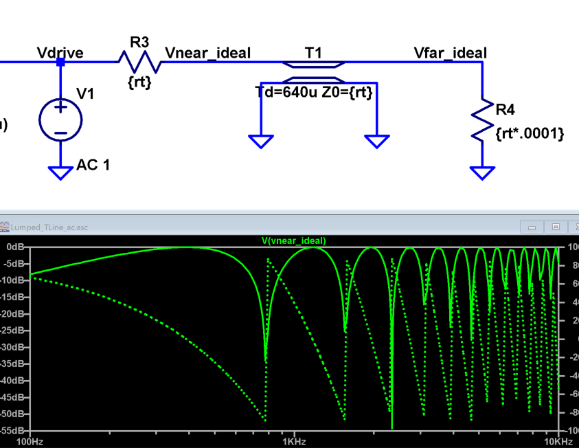
Figure 20. Open can LTspice equivalent
Using the same formula as above, with a frequency approximately 791 Hz and the speed of sound as above, the wavelength in this case is approximately 0.44. Besides the different null frequency, the standing waves pattern in an open cylindric air column also differ. In this case, both ends will be antinodes for the air and thus the length of the column is one half of the wavelength ).
Both measurements gave the same result.
Questions
- If the first null is known, in the given the Network Analyzer frequency response plot, how long is the tube?
Going Further
The Artificial Transmission Lines - ADALM1000 activity includes a complete lumped-element artificial transmission line constructed from capacitors and inductors, as well as detailed measurements of the standing wave patterns along this circuit.
Return to Lab Activity Table of Contents.
university/labs/tlines_standing_waves_adalm2000.txt · Last modified: 01 Nov 2021 18:28 by Mark Thoren