


This version (17 Aug 2016 15:22) was approved by Tom MacLeod.The Previously approved version (16 Aug 2016 20:11) is available.
Table of Contents
ADuCM350 Matlab Model Validation
This page details the work completed to date in evaluating and validating the Matlab/Simulink model of the ADuCM350. Validation work comprises of testing the performance and accuracy of the Matlab model’s measurement results against both the ideal/expected results, and against results from measurements taken directly on an ADuCM350 evaluation board.
The ADuCM350 Matlab model simulates the AFE of the ADuCM350 at a functional block level, allowing voltammetric, amperometric, and impedimetric measurements to be modelled accurately. On both the hardware evaluation board for the ADuCM350 and the Matlab model, the sensor takes the form of an RC impedance network which is separate from the AFE, and can be configured to take the form of an arbitrary RC network. The AFE is connected to the sensor through a programmable switch matrix, which allows changing between 2-Wire and 4-Wire measurements.
RC Impedance Measurement Validation
A primary use case of the ADuCM350 is the measurement of RC impedance networks in a range of frequencies. Numerous experiments are detailed below which were run to validate the Matlab model’s performance in taking these measurements.
Current Level Tests
The figures below show tests of 4-Wire measurements at different current levels through the sensor. Each test was performed on both the model and the hardware, and is shown below compared to the ideal calculated impedance for this particular impedance network. For all current level tests in this section, the sensor was configured as in Figure 2, such that the impedance is: R_SERIES + (R_PARALLEL || C_PARALLEL). R_ACCESS is 1Ω in all measurements in this section.
120 nA


Configuration:
Attenuator: On
V_Excitation: 6.36 mV
R_TIA: 5.6 MΩ
R_Cal: 49.9 kΩ
R_Series: 49.9 kΩ
R_Parallel: 49.9 kΩ
C_Parallel: 1.2 nF
Average Magnitude Error (%):
                           Measured on M350: 1.04
                           Simulated on Model: 2.08
Average Phase Error (%):
                           Measured on M350: 6.20
                           Simulated on Model: 5.33
1 uA
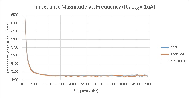

Configuration:
Attenuator: On
V_Excitation: 6.36 mV
R_TIA: 468 kΩ
R_Cal: 5 kΩ
R_Series: 5 kΩ
R_Parallel: 5 kΩ
C_Parallel: 62 nF
Average Magnitude Error (%):
                           Measured on M350: 0.191
                           Simulated on Model: 0.185
Average Phase Error (%):
                           Measured on M350: 7.245
                           Simulated on Model: 9.447
12 uA
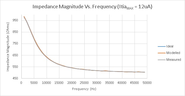

Configuration:
Attenuator: On
V_Excitation: 6.36 mV
R_TIA: 49.6 kΩ
R_Cal: 497 Ω
R_Series: 497 Ω
R_Parallel: 497 Ω
C_Parallel: 62 nF
Average Magnitude Error (%):
                           Measured on M350: 0.202
                           Simulated on Model: 0.172
Average Phase Error (%):
                           Measured on M350: 1.609
                           Simulated on Model: 1.108
200 uA
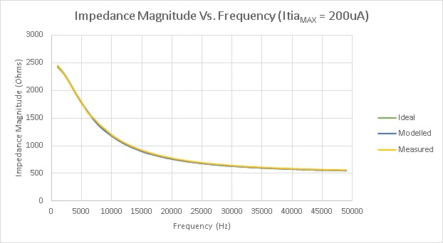

Configuration:
Attenuator: Off
V_Excitation: 100 mV
R_TIA: 3.3 kΩ
R_Cal: 497 Ω
R_Series: 497 Ω
R_Parallel: 1987 Ω
C_Parallel: 16.5 nF
Average Magnitude Error (%):
                           Measured on M350: 1.29
                           Simulated on Model: 0.334
Average Phase Error (%):
                           Measured on M350: 1.33
                           Simulated on Model: 0.546
Summary
For most current ranges tested, the Matlab model marginally outperformed the ADuCM350 hardware measurements. However in nearly every case, the difference between the accuracy of the model and the hardware is small (<1% accuracy difference), indicating that the Matlab model of the ADuCM350 closely replicates the performance of the ADuCM350 in 4-Wire impedance measurements. Also note that for both the hardware and the model, measurement accuracy increases with larger current levels, as the ADuCM350 was designed for measurements involving currents in the hundred-microampere range.
R_ACCESS Tests
Tests were run with varying R_ACCESS in order to validate the operation of the 4-Wire measurements, in which the magnitude of R_ACCESS should have no effect on the measured impedance.
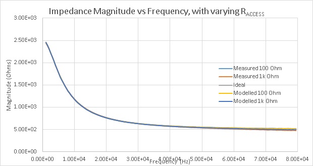
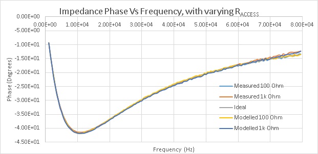
Configuration:
Attenuator: Off
V_Excitation: 100 mV
R_TIA: 3.3 kΩ
R_Cal: 497 Ω
R_Series: 497 Ω
R_Parallel: 1987 Ω
C_Parallel: 16.5 nF
R_ACCESS = 100 Ω

Average Magnitude Error (%):
                           Measured on M350: 0.816
                           Simulated on Model: 0.377
Average Phase Error (%):
                           Measured on M350: 0.798
                           Simulated on Model: 0.743
R_ACCESS = 1 kΩ

Average Magnitude Error (%):
                           Measured on M350: 0.585
                           Simulated on Model: 1.585
Average Phase Error (%):
                           Measured on M350: 0.838
                           Simulated on Model: 1.232
These results indicate that the Matlab model very accurately reproduces the ADuCM350’s 4-Wire measurement capabilities, as the difference in accuracy between the model and the hardware is in all cases ≤ 1%.
2-Wire Tests
The 2-Wire impedance measurement capabilities of the Matlab model are verified against the hardware in the plots below. The sensor impedance for this section is a series resistor and capacitor.


Configuration:
Attenuator: Off
V_Excitation: 200 mV
R_TIA: 10 kΩ
R_Cal: 2000 Ω
R_Series: 2000 Ω
C_Series: 18 nF
Average Magnitude Error (%):
                           Measured on M350: 0.470
                           Simulated on Model: 0.853
Average Phase Error (%):
                           Measured on M350: 7.669
                           Simulated on Model: 2.964
The model achieves better accuracy than the hardware in terms of impedance phase measurement error, and performs very similarly to the hardware in terms of impedance magnitude measurement error.
Noise and Accuracy Validation
Tests were carried out to determine the ideal noise variance level to accurately model the noise levels and measurement accuracy of the ADuCM350 hardware. These tests were carried out both with the attenuator enabled and disabled.
Attenuator On

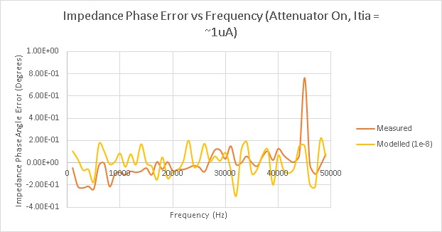
Configuration:
Attenuator: On
V_Excitation: 6 mV
R_TIA: 468 kΩ
R_Cal: 5 kΩ
R_Series: 5 kΩ
R_Parallel: 5 kΩ
C_Parallel: 62 nF
RMS Magnitude Error (Ω):
                           Measured on M350: 15.68
                           Simulated on Model with Var = 1e-8: 11
RMS Phase Error (°):
                           Measured on M350: 0.146
                           Simulated on Model with Var = 1e-8: 0.120
Attenuator Off
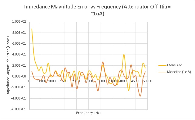

Configuration:
Attenuator: Off
V_Excitation: 6 mV
R_TIA: 468 kΩ
R_Cal: 5 kΩ
R_Series: 5 kΩ
R_Parallel: 5 kΩ
C_Parallel: 62 nF
RMS Magnitude Error (Ω):
                           Measured on M350: 17.23
                           Simulated on Model with Var = 1e-8: 11.71
RMS Phase Error (°):
                           Measured on M350: 0.179
                           Simulated on Model with Var = 1e-8: 0.120
Amperometric Measurement Validation
The amperometric capabilities of the ADuCM350 are available in either Amperometry, Chronoamperomtry, or User Defined modes. The performance of these measurements were validated for both a purely resistive sensor, and an RC sensor. Tests were also conducted with the Sinc2lf filter both disabled and enabled.
Sinc2hf + Sinc2lf Filters Enabled

Configuration:
Attenuator: Off
V_Excitation: Step to 300mV @ t=100ms
R_TIA: 7.5 kΩ
R_Cal: 8.8 kΩ
R_Series: 8.8 kΩ
Measurement Type: 2-Wire
The model and the hardware track very closely for this measurement. The slow rise time is due to the low pass effect of the Sinc2lf filter. Both measurements settle at ~34uA after the voltage step, which is the expected value for the given impedance and step voltage.
Sinc2hf Filter Enabled, Sinc2lf Filter Disabled

Configuration:
Attenuator: Off
V_Excitation: Step to 300mV @ t=100ms
R_TIA: 7.5 kΩ
R_Cal: 8.8 kΩ
R_Series: 8.8 kΩ
Measurement Type: 2-Wire
Again the hardware and the model produce a very similar output for the given input, with both step responses having an identical rise time, settling to their final value after 2 samples.
RC Impedance
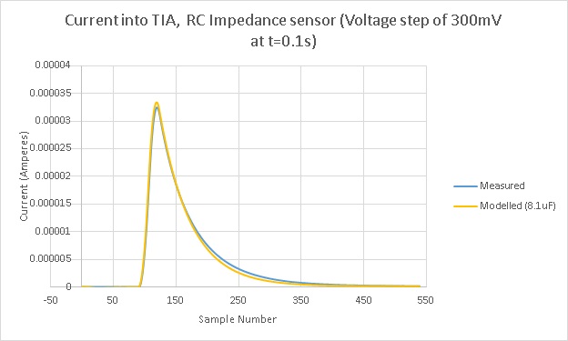
Configuration:
Attenuator: Off
V_Excitation: Step to 300mV @ t=100ms
R_TIA: 7.5 kΩ
R_Cal: 6.8 kΩ
R_Series: 6.8 kΩ
C_Series: 10 uF
Measurement Type: 2-Wire
These plots show visually that the current measurement capabilities of the Matlab model closely match that of the hardware – the difference between the measured and modelled current is typically in the nanoampere-range. Further, the sinc2hf and sinc2lf filters have a nearly identical effect on the model as they do on the hardware.
Amperometric Consistency
All three simulation modes capable of Current Vs. Time measurements should produce the same output, given the same input parameters (The differences between these modes is in the excitation waveforms that are possible with each). The plot below shows the performance of each measurement mode given the same sensor configuration and excitation waveform.

Configuration:
Attenuator: Off
V_Excitation: Step to 600mV for 50ms, step to -300mV for 50ms
R_TIA: 7.5 kΩ
R_Cal: 1 kΩ
R_Series: 6.8 kΩ
C_Series: 10 uF
Measurement Type: 4-Wire
Footnote
All tests were carried out with high-accuracy passive components where possible, however some discrepancies between ideal, measured, and modelled results may be partly due to inaccuracies in the components used in measurements taken on the ADuCM350 evaluation board hardware.
resources/technical-guides/model_aducm350/validation.txt · Last modified: 17 Aug 2016 10:22 by Dylan Stuart