


This version is outdated by a newer approved version. This version (12 Oct 2016 16:44) is a draft.
Approvals: 0/1The Previously approved version (13 Sep 2016 13:11) is available.
This version (12 Oct 2016 16:44) is a draft.Approvals: 0/1The Previously approved version (13 Sep 2016 13:11) is available.
This is an old revision of the document!
Table of Contents
New landing page for ADuCM350 Simulink model.
Getting Started
1. Getting MathWorks' Licenses
2. Opening the Model
Begin by opening Matlab. The Matlab environment will begin on opening and a Matlab command window and workspace will be displayed. To open the model, click on the “Browse for Folder” icon near the top left corner of the window.

A modal window will open, allowing you to browse to the directory where the model is saved. Once you’ve navigated to the right directory, click “Select Folder” on the modal.
If you’ve selected the right folder, a list of files, including the ADuCM350 Model, will appear in the “Current Folder” panel of the Matlab environment window.

The model file should be named
ADuCM350_<version>.slx
and double clicking it will launch Simulink and load the model file so that you can run simulations. Simulink may take up to a few minutes to launch. Once Simulink has loaded the model, it will open in a new window and display some blocks of the model. The model explorer bar, running across the top of the model view, will show the current model block being viewed. For now, we’re only interested in the top level view.

If the model explorer bar shows that you are viewing a lower level block, click on the “ADuCM350_<version>” label in the explorer bar to get back to the top level.
2. Configuring the Sensor
The sensor block contains the passive impedance components which model the electrical characteristics of a real-world electrochemical or biochemical sensor, so configuring it correctly will ensure that your simulation results are accurate and meaningful. The sensor block can be navigated to by double clicking it in the Simulink window.
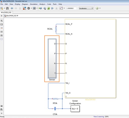
Inside the block, you can see the passive components that make up the sensor. For most applications, these will be capacitors and resistors in various configurations, however they are completely user-configurable.
You can select a component by clicking on it, and standard keyboard shortcuts apply (Copy, Cut, Paste, etc.). Right clicking a component brings up further options for the component, and double clicking a component opens a modal window, from where you can edit the component's parameters.
3. Running a Simulation
Once the sensor is set up in the appropriate configuration, the rest of the model parameters may be set up so that a simulation can be run. In the top level view of the model, the simulation settings can be setup by double clicking on the large block labelled “ADuCM350”, which will bring up a modal window allowing you to edit the block parameters. The modal also gives some information about the device.
3.1. General Simulation Setup
There are four main types of measurement that can be run on the model:
The measurement mode can be selected by clicking on the drop down selection box labelled “Mode” in the ADuCM350 modal. Once you’ve selected the measurement mode, please see the relevant section on configuring the simulation parameters for that mode before continuing.
3.2. Configuring RTIA
Once the settings have been configured for the measurement type selected, the Trans-Impedance Amplifier (TIA) can be set up using RTIA, which is seen in the top level view of the model. At this stage the excitation voltage should be configured from when the measurement mode parameters were set. If not, please see Section 4, 5, or 6 to configure the measurement mode. Knowing the maximum excitation voltage, the value of RTIA can be calculated as follows:
RTIA = (0.75V x Z_SENSOR)/V_EXCITATION
Where ZSENSOR is the minimum value that the sensor impedance will take in the frequency range you are measuring. This calculation gives an upper bound on the value of RTIA. A value slightly lower than this should be used to ensure that the ADC voltage is always less than 750mV (The maximum ADC range) – a safety factor of 1.2 is recommended, so if the ideal value of RTIA is calculated to be 1.2kΩ, use a value of 1kΩ (See Application Note AN-1302: 4_wire_bio_isolated for further reading on RTIA calculation).
3.3. Setting the Attenuation, Switch Mux Configuration, and Filter Options
The attenuation parameter in the settings tab of the ADuCM350 block sets the gain of the Programmable Gain Amplifier (PGA) in the model. It has two settings: 1 (non-attenuator mode) or 0.025 (attenuator mode).
Setting the PGA to attenuator mode has the benefit of providing greater resolution (DAC LSB is 40 times smaller) for the excitation voltage, the trade-off being that the maximum peak voltage of the excitation stage is also 40 times smaller (600mV x 0.025 = 15mV maximum VPK). If attenuator mode is chosen, ensure that the maximum sense voltage is no greater than 15mV, otherwise the simulation will fail the voltage check and an error dialogue will show.
The Switch Matrix Configuration parameter can be configured so that a 2-Wire or 4-Wire measurement is taken, or so that a measurement is taken across RCAL.
For the Filter Options, the ADuCM350 is most commonly used with both the Sinc2hf and Sinc2lf filters enabled, though the option exists to disable the Sinc2lf 50/60Hz supply rejection filter. The model also gives the option to disable both filters, however this option does not exist on the actual ADuCM350 hardware.
3.4. Selecting the Simulation Mode
Once the simulation settings have been configured, click “OK” on the modal to get back to the top view of the model. At the top of the window, you’ll find a drop down selection box which allows you to choose the Simulation Mode.

We recommend using Accelerator mode for running simulations on this model. More information about Simulink simulation modes can be found on the MathWorks website.
3.5. Running the Simulation
To run the simulation, simply click the green “Run” button on the toolbar.

Simple simulations can take a few seconds to run (e.g. single frequency impedance measurements, short amperometric measurements), while longer or more granular simulations have no upper bound on their run time (e.g. amperometric measurements can run through unlimited periods, impedance measurement sweeps can take very small increments), though for most purposes simulations should take no longer than 10 or 15 minutes on a modern PC. Once the simulation is complete, a plot will appear in a separate window showing the simulation results.
3.6. Analyzing the Simulation Results
The plots produced by the simulations provide a good visual mechanism to quickly interpret the results. For further analysis, the outputs of the simulation are stored in variables in the Matlab “Workspace”, accessible in the main Matlab window. For impedance measurement simulations, the magnitude of the impedances are stored in the “mags” variable with unit Ohms, and the phase/arguments of the impedances are stored in the “args” variable with unit Degrees. For current measurement simulations (Amperometric, Chronoamperometric, User Defined), the resulting sampled current values in Amperes are stored in the “mags” variable. These variables hold column vectors of the results which can be seen by double clicking on the variable name. The results can be analysed further using Matlab, or by copying them into another analysis tool (e.g. Excel).
4. Impedance Measurements
To run an impedance measurement simulation, select “Impedance of Sensor (Sinusoid)” as the Mode in the measurement dialogue.

You now have several options for the measurement. The Sense Voltage can have a maximum value of 600mV (Note that this maximum is as seen by the sensor, so different sensor and access impedance configurations may reduce the maximum allowable sense voltage – a headroom check in the model will produce an error if the sense voltage is too large). The Capture Mode can be set so that the impedance is measured:
- At a single frequency (“Single”)
- Through a range of frequencies (“Sweep”)
- At a single frequency, multiple times (“Continuous”)
Depending on which Capture Mode is selected, the sinusoid frequencies can easily be entered accordingly. The delay time for settling can also be set. Once all of the simulation parameters have been configured, click “OK” to save the settings.
In the top level view of the model, three additional passive components can be seen. RCAL is the calibration resistor, which is used when making a ratiometric impedance measurement. Set RCALs value to the lowest impedance value you expect the sensor to take for the frequencies you’ll be measuring at. For example, if you’re measuring a 1nF capacitor in series with a 2kΩ resistor from 1kHz to 50kHz, RCAL should be set as follows:
RCAL = |2000Ω+ 1/(j(2π50,000Hz)(1e-9F))| ≈ 3760Ω
Once RCAL is set, continue reading Section 3.1 to run the simulation.
5. Amperometric Measurements
To run an amperometric measurement simulation, select “Amperometry” as the Mode in the measurement dialogue.

You now have several options for the measurement. The diagram explains the excitation waveform which will be forced across the sensor, and its configurable parameters.
Single Capture mode will cycle through a single period of the trapezoid waveform, while Continuous Capture mode allows multiple periods of the trapezoidal waveform to be run.
Once the measurement settings are configured, continue reading Section 3.1 to run the simulation.
6. Chronoamperometric Measurements
To run a chronoamperometric measurement simulation, select “Chronoamperometry” as the Mode in the measurement dialogue.

You now have several options for the measurement. The diagram explains the excitation waveform which will be forced across the sensor, and its configurable parameters.
The number of periods (E1 to E2 cycles) can also be configured in the dialogue.
Once the measurement settings are configured, continue reading Section 3.1 to run the simulation.
7. User Defined Measurements
To run a user defined measurement simulation, wherein the excitation waveform is arbitrarily customisable by the user, select “User Defined” as the Mode in the measurement dialogue.

You now have several options for the measurement. The diagram explains the excitation waveform which will be forced across the sensor, and its configurable parameters. The waveform is defined by inputting a series of “Potential, Time” points, as seen in the measurement dialogue. When the simulation is run, a linear interpolation between these points is performed to generate the excitation waveform, meaning any arbitrary excitation waveform is possible.
Once the measurement settings are configured, continue reading Section 3.1 to run the simulation.
Validation
Please go to the ADuCM350 Matlab Model Validation page for information on the validation work done to verify the accuracy of the model.
resources/technical-guides/model_aducm350.1476283490.txt.gz · Last modified: 12 Oct 2016 16:44 by Tom MacLeod